



Click Below to Get the Code

Browse, clone, and build from real-world templates powered by Harper.
Comparison
GitHub Logo

Faster Vector Search in Harper 5.3 with Native HNSW

Explore vector index in Harper 5.3’s with benchmarks against pgvector and Harper 5.2, and the open-source Node.js package @harperfast/hnsw.
Comparison

Faster Vector Search in Harper 5.3 with Native HNSW

Kris Zyp
SVP of Engineering
at Harper
October 8, 2026
Kris Zyp
SVP of Engineering
at Harper
October 8, 2026
Kris Zyp
SVP of Engineering
at Harper
October 8, 2026
October 8, 2026
Explore vector index in Harper 5.3’s with benchmarks against pgvector and Harper 5.2, and the open-source Node.js package @harperfast/hnsw.
Kris Zyp
SVP of Engineering

Vector search becomes expensive when a query has to visit thousands of graph nodes, and each visit means loading a record, decoding it, and managing JavaScript objects. Faster distance calculations help, but graph traversal and memory access can account for much of the work.

Harper 5.3 introduces a native HNSW index built around a persistent, memory-mapped graph. The implementation is also available as the open-source @harperfast/hnsw module for Node.js. We moved the search loop and its data layout together: vectors and neighbors live in fixed-size slots, and Rust traverses those slots on native threads.

We benchmarked the released Harper 5.3.0 against Harper 5.2.15 and PostgreSQL 17.11 with pgvector 0.8.7. On 20,000 vectors, 5.3 delivered 3.7x the throughput of 5.2 at approximately 99% recall, and 6.5x at 99.95% recall. On 200,000 vectors, 5.3 delivered about 1.6x the throughput of similar stack using pgvector. The comparisons include the HTTP request, query execution, and response, with recall measured against exact nearest neighbors.

Why move the graph into a native module?

HNSW, or Hierarchical Navigable Small World, organizes vectors in a graph. A search starts in the upper layers to find a useful neighborhood, then explores more candidates in the bottom layer. It avoids comparing the query with every vector, in exchange for occasionally missing a true nearest neighbor.

Harper 5.2 stores graph nodes through the database's record layer and searches them in JavaScript. Caching helps considerably, but each visited node still participates in the JavaScript search machinery: candidate heaps, visited sets, neighbor iteration, and object access.

The new module stores the traversal graph in a memory-mapped file. A node's quantized vector and neighbor IDs sit together in a fixed-size slot. Native traversal can address that slot directly, avoiding a database lookup and record decode at each visit. Distance calculations use SIMD where supported, and candidate and visited-node tracking stay in native code. JavaScript handles the request and the records returned to the application.

This also gives the index a useful persistence model. A compatible graph can be mapped again when reopened, without deserializing the whole graph into JavaScript objects. Inserts, updates, and deletes maintain the graph incrementally. Searches and writes coordinate through per-slot sequence locks rather than a global search lock. The implementation and its tradeoffs are described in the module's design notes.

Comparing speed at the same recall

An approximate index can answer faster by exploring less of its graph. Throughput only means something alongside the fraction of true neighbors it finds.

We measure recall@10: the fraction of the exact ten nearest neighbors that appear in the ten results. A recall of 99.5% means the index returned 9.95 of those neighbors per query on average. It does not mean that every query returned all ten.

Our corpus is SIFT descriptors with 128 dimensions. These are real image descriptors, rather than random vectors. We use cosine distance and recompute exact neighbors for each indexed subset. Standard SIFT benchmark results usually use Euclidean distance, but cosine distances are used more frequently in real applications.

Harper uses six server workers. The pgvector endpoint uses six Fastify workers backed by PostgreSQL connections. Both stacks are restricted to one hardware thread on each of six physical performance cores. Four HTTP client workers run on separate efficiency cores, with 32 concurrent requests in total. We sweep the search budget, ef, and measure warm queries. All runs use the same XPS laptop, Node.js 24.21.0, and local NVMe storage.

Harper 5.3 versus 5.2

For the three-system comparison, we indexed 20,000 vectors and used 200 query vectors. Each search-budget setting ran 10,000 requests, repeating those query vectors 50 times.

HTTP benchmark: 20,000 vectors
SystemSearch budget (ef)Recall@10Queries/secMedian latencyp99 latency
Harper 5.3.04099.50%4,6265.69 ms18.66 ms
Harper 5.2.154099.35%1,25824.54 ms44.91 ms
pgvector 0.8.74099.50%4,3016.17 ms24.31 ms

These are each system's first measured settings above 99% recall. Harper 5.3 returned slightly more true neighbors than 5.2 while delivering 3.7 times the throughput. At this accuracy and corpus size, Harper 5.3 and pgvector were close: the measured throughput difference was about 8%. We would treat that as competitive performance, rather than a decisive advantage from one run.

The gap between Harper versions grows when we ask for more accuracy. At ef=80, both versions achieved 99.95% recall. Harper 5.3 delivered 4,258 queries/sec versus 652 for 5.2, a 6.5x improvement. Median latency was 6.30 ms versus 47.19 ms at the same request concurrency.
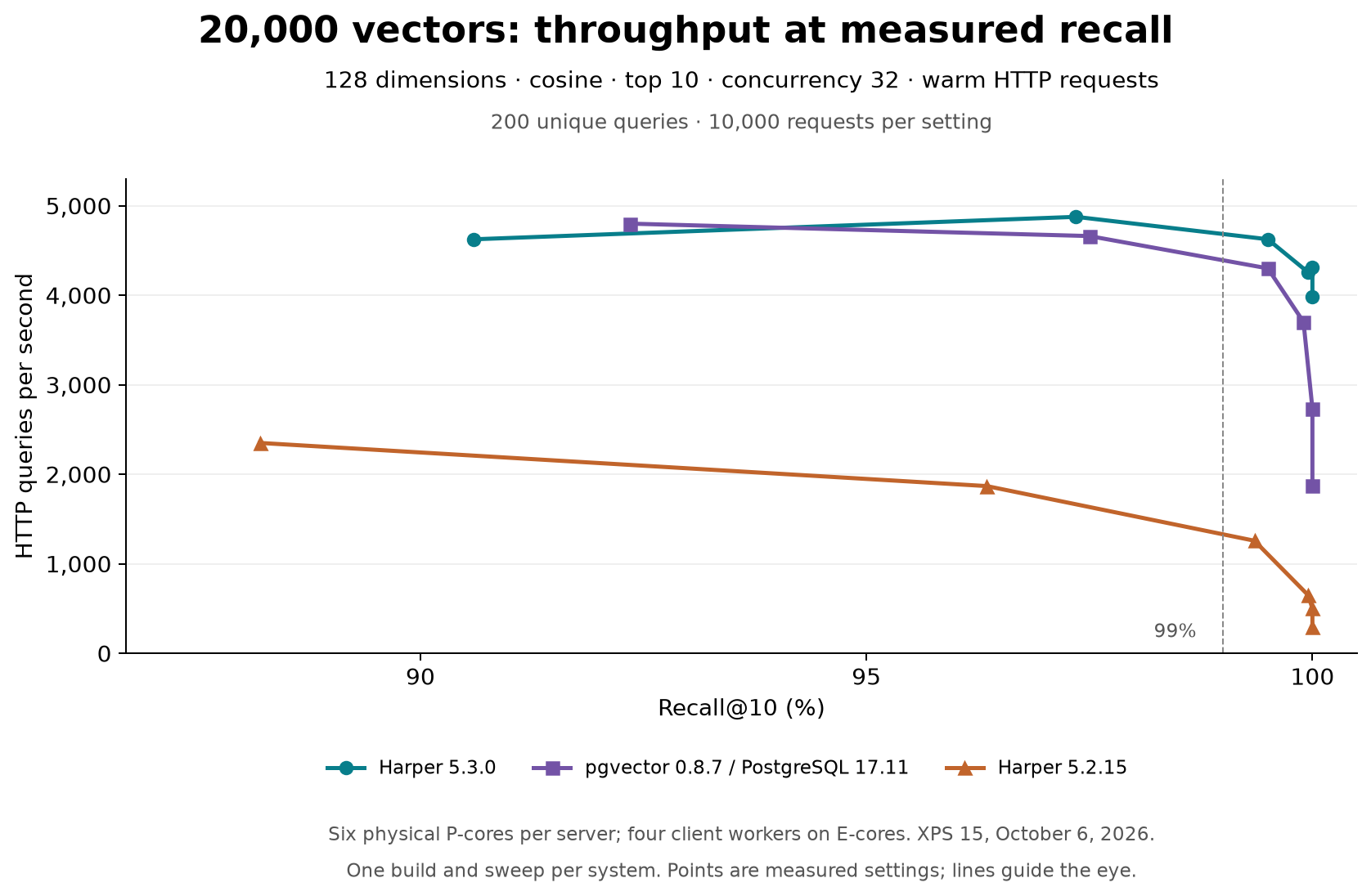
HTTP query throughput versus recall@10 on 20,000 vectors. Harper 5.3 and pgvector perform similarly near 99% recall, while Harper 5.3 maintains higher throughput as recall approaches 100%. Harper 5.2 is slower throughout the measured range.

Comparing with pgvector on a larger corpus

We then increased the corpus to 200,000 vectors and used 500 query vectors, repeated 20 times per setting. This run compares Harper 5.3 and pgvector; we did not measure Harper 5.2 at this size. The CPU allocation and request concurrency stayed the same.

HTTP benchmark: 200,000 vectors
SystemSearch budget (ef)Recall@10Queries/secMedian latencyp99 latency
Harper 5.3.08099.22%4,0216.65 ms23.75 ms
pgvector 0.8.78099.14%2,51310.97 ms38.74 ms
Harper 5.3.016099.84%3,8196.80 ms23.65 ms
pgvector 0.8.716099.82%1,69517.19 ms50.91 ms

Both systems needed a larger search budget to reach 99% recall on this corpus. At their first measured settings above 99%, Harper delivered 1.6x pgvector's throughput. Above 99.8%, that ratio was 2.3 times, with closely matched measured recall. These are the results of this workload and configuration, rather than a general ranking of vector databases.
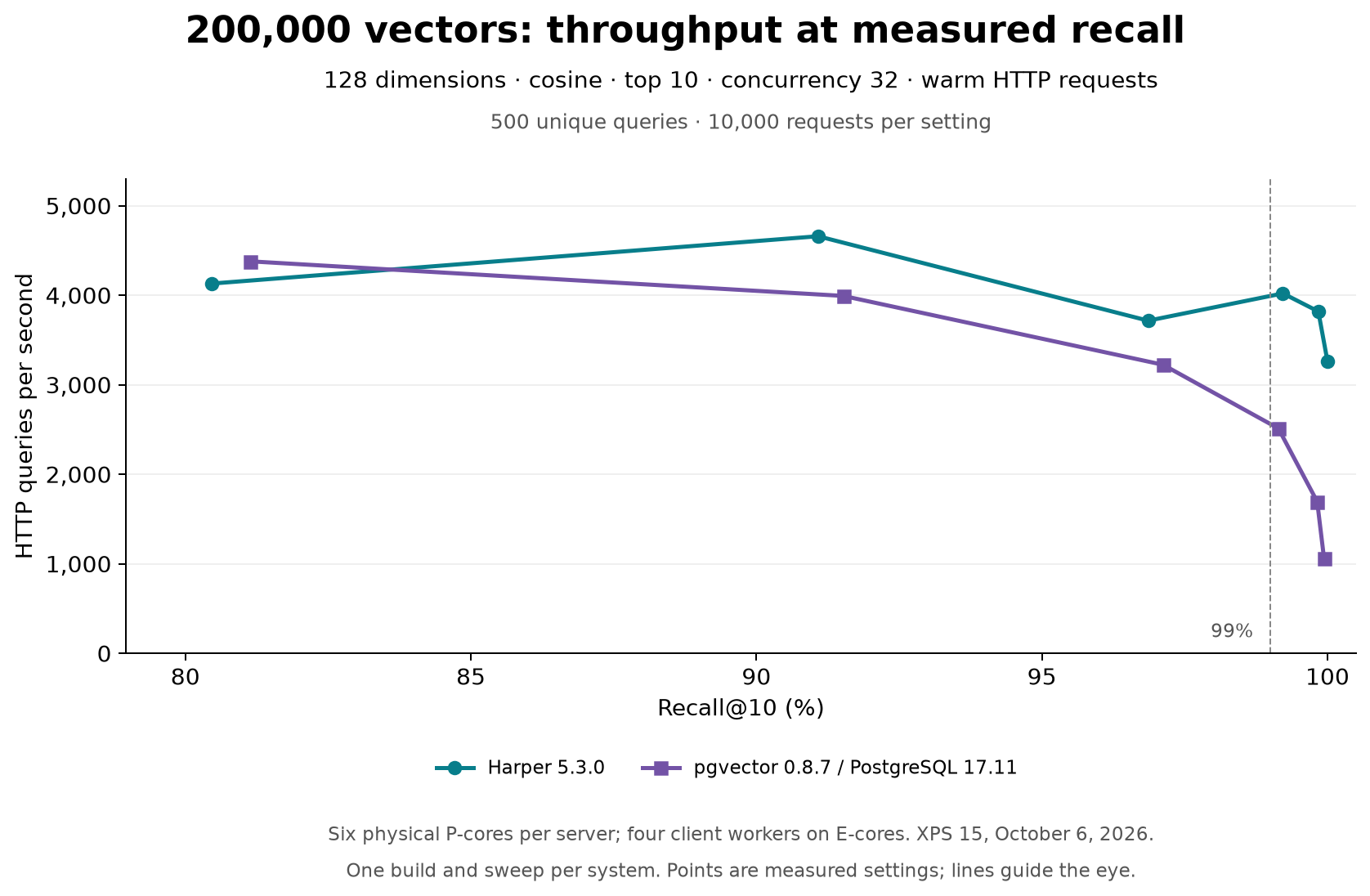
HTTP query throughput versus recall@10 on 200,000 vectors. Near 99% recall, Harper 5.3 achieves about 4,000 queries per second versus 2,500 for pgvector. As recall approaches 100%, throughput drops to approximately 3,300 and 1,100 queries per second, respectively.

Each point is one search-budget setting. Lines connect measured points; they do not estimate unmeasured settings. The small reversals in throughput reflect timing variability in these individual sweeps.

Fastify and HTTP overhead

We checked the HTTP adapter separately using the same 200,000-vector index at ef=160, with 32 concurrent requests and three rounds per path. Replacing Fastify with a minimal Node.js HTTP handler, while keeping the six server workers, PostgreSQL driver, SQL, and CPU allocation the same, increased mean throughput from 1,729 to 1,775 queries/sec: only about 2.7%. An HTTP control that parsed the same vector payload and returned ten IDs without querying PostgreSQL handled about 6,107 requests/sec.

The complete HTTP adapter has a larger cost. In a separate three-round comparison, direct PostgreSQL requests averaged 2,362 queries/sec versus 1,722 through Fastify, a 37% increase. The main results compare complete HTTP search paths; Fastify's own contribution was small in this diagnostic (again, about 2.7%).

Quantization and the cost of accuracy

Harper's native traversal stores vectors as int8 values. That reduces the bytes a graph visit needs to read, but introduces approximation into distance calculations. Harper then calculates full-precision distances for a bounded candidate set before returning results. For an unfiltered top-10 native query, the current implementation reranks up to 40 candidates, subject to the search budget.

This separation matters as accuracy increases. A larger ef gives native traversal more room to find useful candidates without requiring a full record load for every visited node. PostgreSQL's index in this comparison stores float32 vectors. The implementations make different choices about representation and traversal, which is why measured recall is the comparison point.

The right budget depends on the corpus. A setting that works well for 128-dimensional image descriptors may behave differently for 768- or 1,536-dimensional text embeddings. Measure against exact neighbors from your own data before choosing it.

Using the native index in Harper

A new eligible HNSW declaration in Harper 5.3 selects the native backend automatically. The table must use RocksDB with auditing enabled, and the index must use the supported cosine, int8, and default structural settings. For example:

type Document @table @export {
	id: ID @primaryKey
	text: String
	embedding: [Float] @indexed(type: "HNSW", distance: "cosine")
}

The query surface stays the same:

const response = await fetch('/Document/', {
	method: 'QUERY',
	headers: { 'Content-Type': 'application/json' },
	body: JSON.stringify({
		sort: {
			attribute: 'embedding',
			target: queryVector,
			distance: 'cosine',
			ef: 80,
			waitForIndexMilliseconds: 30_000,
		},
		limit: 10,
		select: ['id', 'text'],
	}),
});

Native indexing follows committed writes asynchronously. waitForIndexMilliseconds lets a query wait for the index to cover local writes committed before the search begins; a rebuilding or unavailable index can still refuse the query. RocksDB records and the audit history are the recovery source, while the graph file is derived state that Harper can rebuild or catch up.

Existing indexes retain the backend they were built with. An upgrade alone therefore does not convert an existing JavaScript graph into a native graph. Unsupported configurations continue to use the previous backend when nativePlane is unset; an explicit local nativePlane: true declaration is rejected when ineligible. See the Harper 5.3 release notes for the selection and upgrade rules.

Using @harperfast/hnsw directly

The native engine is also available independently of Harper. We have open-sourced HarperFast/hnsw under the Apache 2.0 license. It provides a persistent cosine-similarity index for Node.js, with graph traversal implemented in Rust. You can use it in an application that manages its own records and embeddings.

The measurements below use version 0.4.0. Install that version with Node.js 22 or later:

npm install @harperfast/hnsw@0.4.0

Here is a small example using three-component vectors and application record keys. Save it as example.cjs and run node example.cjs:

const { Plane } = require('@harperfast/hnsw');
const { existsSync } = require('node:fs');

async function main() {
	const path = './vectors.hnsw';
	if (existsSync(path)) throw new Error('Use a fresh path for Plane.create');
	const plane = Plane.create(path, 3, 64, 100_000, 32);
	plane.insert(new Float32Array([1, 0, 0]), Buffer.from('article:1'));
	plane.insert(new Float32Array([0.8, 0.2, 0]), Buffer.from('article:2'));
	plane.insert(new Float32Array([0, 1, 0]), Buffer.from('article:3'));
	await plane.flushAsync();

	const hits = await plane.search(new Float32Array([1, 0, 0]), 2, 80);
	for (let i = 0; i < hits.ids.length; i++) {
		const start = i === 0 ? 0 : hits.keyEnds[i - 1];
		const key = hits.keys.subarray(start, hits.keyEnds[i]).toString();
		console.log(key, hits.distances[i]);
	}
}

main();

The creation arguments specify the file path, three dimensions, a layer-0 neighbor capacity of 64, space for up to 100,000 nodes, and 32 inline bytes per record key. The node capacity is a sparse reservation: pages are allocated as the index is populated. Real applications would use the dimensionality of their embedding model. On a later startup, reopen the file with Plane.open('./vectors.hnsw'). Plane.create replaces an existing file, which is why the example checks the path first.

search(query, k, ef) returns the nearest k candidates in parallel typed arrays, ordered by approximate cosine distance. Here k=2 and ef=80; increasing ef spends more work exploring the graph. Search runs asynchronously on Node's native thread pool. The returned keys let the application retrieve its records. For bulk loading, insertBatch accepts a flat, row-major Float32Array, optional concatenated key bytes and key offsets, and a native thread count. Await each chunk, inspect rejected records, and await all inserts before flushing. Keep the returned node IDs if you need to delete entries with remove(id). The API reference describes these operations.

The package stores the graph and quantized vectors; the application retains its records and any original vectors needed for exact reranking or rebuilding. By default, storage precision is int8. To create an int16 index, pass 'int16' as the seventh argument:

const plane = Plane.create('./vectors-int16.hnsw', 128, 64, 100_000, 32, undefined, 'int16');

Int16 adds one byte per dimension to each stored vector. It gives finer distance estimates, but whether you can omit exact reranking depends on your corpus. Precision is fixed when the file is created. These are standalone package options; Harper's native integration currently uses int8 with exact reranking.

Isolated package benchmarks: 20,000 vectors

We also measured the package directly, using the same XPS machine, 128-dimensional SIFT subsets, cosine ground truth, and top 10. These calls include the Node/native boundary and result allocation. They exclude HTTP, database record access, and exact reranking.

One mode uses searchSync from one calling thread; this blocks that thread and is useful as a baseline. The other keeps six asynchronous search calls in flight, with UV_THREADPOOL_SIZE=6. The entire process, including the Node event loop and native threads, shares the same six performance cores.

Standalone package: 20,000 vectors
PrecisionSearch budgetRecall@10One caller QPSOne caller medianSix concurrent searches QPS
int88098.35%7,6670.131 ms22,859
int168099.95%7,6480.132 ms21,218

At this setting the two builds have similar latency from one caller, while int16 returns more of the exact neighbors. Raw int8 recall levels off at 98.35% through ef=320. Increasing the search budget alone does not remove the error in the stored distances.
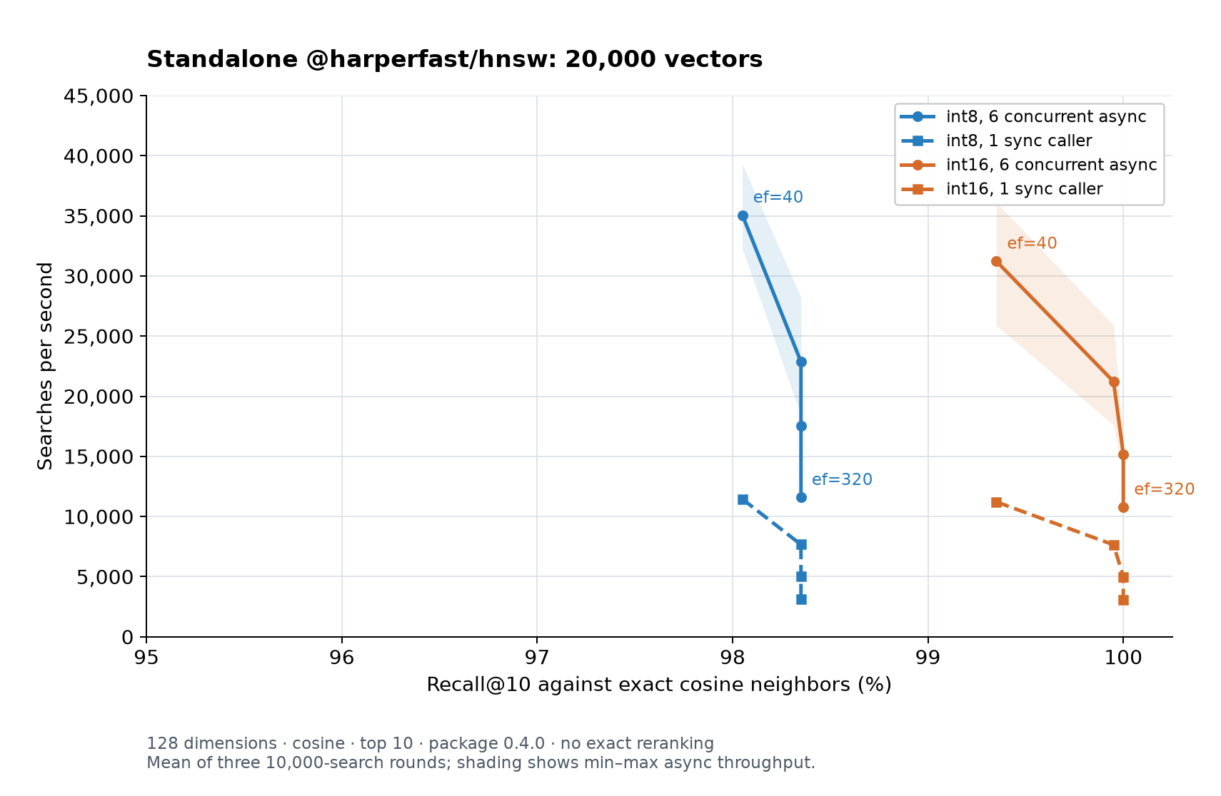
Search throughput versus recall@10 for standalone @harperfast/hnsw on 20,000 vectors. Int8 reaches about 98.4% recall; int16 reaches 100%. Six concurrent asynchronous searches deliver higher throughput than one synchronous caller, with throughput declining as the search budget increases.

Isolated package benchmarks: 200,000 vectors

Standalone package: 200,000 vectors
PrecisionSearch budgetRecall@10One caller QPSOne caller medianSix concurrent searches QPS
int816097.68%2,9680.340 ms11,437
int1616099.84%2,9460.346 ms9,531
int832097.82%1,8570.550 ms6,757
int16320100.00%1,7970.568 ms6,008

Int16 finds all exact top-10 neighbors for these 500 queries at ef=320; that is a result for this finite query set. The int8 build reaches 97.82% at the same budget. This is why a standalone application should evaluate precision and exact reranking together with its search budget.
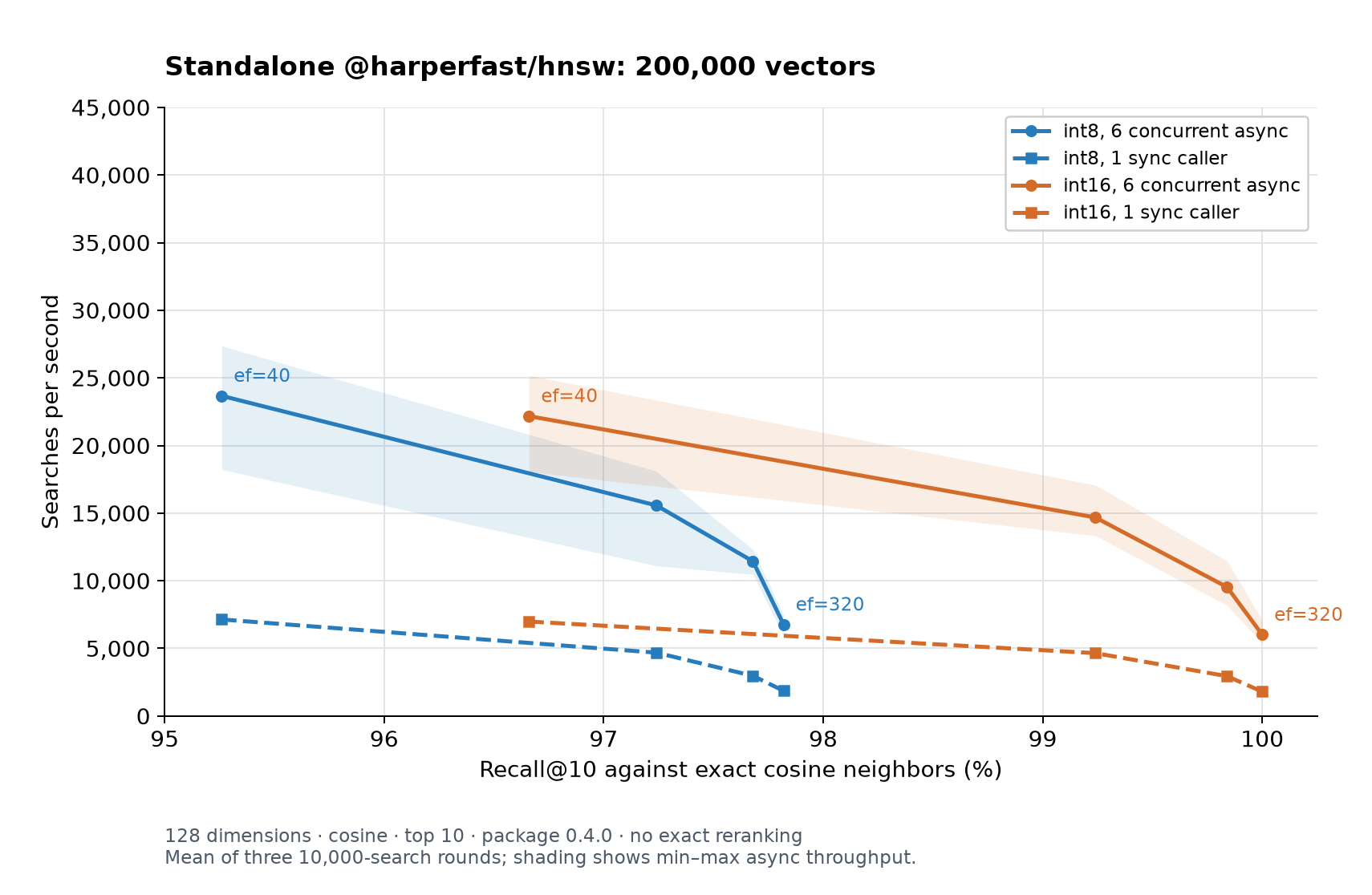
Search throughput versus recall@10 for standalone @harperfast/hnsw on 200,000 vectors. Int8 reaches about 97.8% recall; int16 reaches 100%. Six concurrent asynchronous searches deliver higher throughput than one synchronous caller, with throughput declining as the search budget increases.

Both corpus sizes use freshly built indexes, layer-0 capacity 64, no embedded record keys, and the package's native builder with M=16 and efConstruction=200. We built each index in chunks of 10,000 vectors with six insertion threads. Inserting 200,000 vectors took 13.6 seconds for each precision, with the final durability flush measured separately.

Each plotted point averages three rounds of 10,000 searches after warm-up; the latency column averages the three round medians. Recall uses 200 unique queries at 20,000 vectors and 500 at 200,000 vectors. We repeated timing on one build per precision and size. Concurrent throughput varied substantially between rounds on this shared machine: for example, the 200,000-vector int16 case at ef=160 ranged from 8,176 to 11,468 QPS. The complete ranges are in the benchmark data.

These measurements use the package's own graph builder and omit Harper's record handling and reranking. The earlier HTTP measurements cover a different execution path and concurrency level; dividing the two throughputs would not isolate HTTP overhead.

What these measurements cover

These are unfiltered, warm, top-10 searches on one laptop. The database comparisons include application and transport costs, and the pgvector result includes the Fastify application exposing its HTTP endpoint. They do not measure cold storage, an index larger than RAM, concurrent mutations, replication, embedding generation, or retrieval quality in a complete RAG application.

The dataset and query count also limit the conclusion. Repeating requests improves timing measurement, but does not create additional independent recall samples. A finite sample reporting 100% recall is not a guarantee of perfect recall on future queries. We ran one index build and one sweep per database and corpus size; the standalone package timings and HTTP diagnostics repeat three rounds on fixed builds. We did not calculate confidence intervals. CPU placement is controlled, but the computer still runs other work and changes frequency. Treat small percentage differences cautiously.

Search throughput is also only part of performance. For the 20,000-vector corpus, time to load and make the index queryable was 8.7 seconds for Harper 5.3, 91.3 seconds for Harper 5.2, and 4.3 seconds for PostgreSQL with pgvector. The two Harper versions used the same REST ingestion path; PostgreSQL used COPY followed by a bulk index build. PostgreSQL was faster at this initial-load task, while Harper's new implementation substantially reduced the time spent on initial ingestion and indexing. For 200,000 vectors, Harper 5.3 took 94.2 seconds to load and become queryable; PostgreSQL with pgvector took 39.7 seconds.

The module gives us a more direct path from a query to the graph data it needs, while retaining a persistent index that can be maintained as records change. Its next performance tests should cover wider embeddings, selective metadata filters, and datasets large enough to put pressure on memory.

Benchmark data

The HNSW benchmark methodology including isolated package tests and HNSW benchmark evidence including isolated package tests include the complete search-budget sweeps, runtime versions, hardware configuration, and benchmark harnesses for the database comparisons, HTTP diagnostics, and standalone package tests. All measurements were taken on October 6, 2026.

‍

Vector search becomes expensive when a query has to visit thousands of graph nodes, and each visit means loading a record, decoding it, and managing JavaScript objects. Faster distance calculations help, but graph traversal and memory access can account for much of the work.

Harper 5.3 introduces a native HNSW index built around a persistent, memory-mapped graph. The implementation is also available as the open-source @harperfast/hnsw module for Node.js. We moved the search loop and its data layout together: vectors and neighbors live in fixed-size slots, and Rust traverses those slots on native threads.

We benchmarked the released Harper 5.3.0 against Harper 5.2.15 and PostgreSQL 17.11 with pgvector 0.8.7. On 20,000 vectors, 5.3 delivered 3.7x the throughput of 5.2 at approximately 99% recall, and 6.5x at 99.95% recall. On 200,000 vectors, 5.3 delivered about 1.6x the throughput of similar stack using pgvector. The comparisons include the HTTP request, query execution, and response, with recall measured against exact nearest neighbors.

Why move the graph into a native module?

HNSW, or Hierarchical Navigable Small World, organizes vectors in a graph. A search starts in the upper layers to find a useful neighborhood, then explores more candidates in the bottom layer. It avoids comparing the query with every vector, in exchange for occasionally missing a true nearest neighbor.

Harper 5.2 stores graph nodes through the database's record layer and searches them in JavaScript. Caching helps considerably, but each visited node still participates in the JavaScript search machinery: candidate heaps, visited sets, neighbor iteration, and object access.

The new module stores the traversal graph in a memory-mapped file. A node's quantized vector and neighbor IDs sit together in a fixed-size slot. Native traversal can address that slot directly, avoiding a database lookup and record decode at each visit. Distance calculations use SIMD where supported, and candidate and visited-node tracking stay in native code. JavaScript handles the request and the records returned to the application.

This also gives the index a useful persistence model. A compatible graph can be mapped again when reopened, without deserializing the whole graph into JavaScript objects. Inserts, updates, and deletes maintain the graph incrementally. Searches and writes coordinate through per-slot sequence locks rather than a global search lock. The implementation and its tradeoffs are described in the module's design notes.

Comparing speed at the same recall

An approximate index can answer faster by exploring less of its graph. Throughput only means something alongside the fraction of true neighbors it finds.

We measure recall@10: the fraction of the exact ten nearest neighbors that appear in the ten results. A recall of 99.5% means the index returned 9.95 of those neighbors per query on average. It does not mean that every query returned all ten.

Our corpus is SIFT descriptors with 128 dimensions. These are real image descriptors, rather than random vectors. We use cosine distance and recompute exact neighbors for each indexed subset. Standard SIFT benchmark results usually use Euclidean distance, but cosine distances are used more frequently in real applications.

Harper uses six server workers. The pgvector endpoint uses six Fastify workers backed by PostgreSQL connections. Both stacks are restricted to one hardware thread on each of six physical performance cores. Four HTTP client workers run on separate efficiency cores, with 32 concurrent requests in total. We sweep the search budget, ef, and measure warm queries. All runs use the same XPS laptop, Node.js 24.21.0, and local NVMe storage.

Harper 5.3 versus 5.2

For the three-system comparison, we indexed 20,000 vectors and used 200 query vectors. Each search-budget setting ran 10,000 requests, repeating those query vectors 50 times.

HTTP benchmark: 20,000 vectors
SystemSearch budget (ef)Recall@10Queries/secMedian latencyp99 latency
Harper 5.3.04099.50%4,6265.69 ms18.66 ms
Harper 5.2.154099.35%1,25824.54 ms44.91 ms
pgvector 0.8.74099.50%4,3016.17 ms24.31 ms

These are each system's first measured settings above 99% recall. Harper 5.3 returned slightly more true neighbors than 5.2 while delivering 3.7 times the throughput. At this accuracy and corpus size, Harper 5.3 and pgvector were close: the measured throughput difference was about 8%. We would treat that as competitive performance, rather than a decisive advantage from one run.

The gap between Harper versions grows when we ask for more accuracy. At ef=80, both versions achieved 99.95% recall. Harper 5.3 delivered 4,258 queries/sec versus 652 for 5.2, a 6.5x improvement. Median latency was 6.30 ms versus 47.19 ms at the same request concurrency.

HTTP query throughput versus recall@10 on 20,000 vectors. Harper 5.3 and pgvector perform similarly near 99% recall, while Harper 5.3 maintains higher throughput as recall approaches 100%. Harper 5.2 is slower throughout the measured range.

Comparing with pgvector on a larger corpus

We then increased the corpus to 200,000 vectors and used 500 query vectors, repeated 20 times per setting. This run compares Harper 5.3 and pgvector; we did not measure Harper 5.2 at this size. The CPU allocation and request concurrency stayed the same.

HTTP benchmark: 200,000 vectors
SystemSearch budget (ef)Recall@10Queries/secMedian latencyp99 latency
Harper 5.3.08099.22%4,0216.65 ms23.75 ms
pgvector 0.8.78099.14%2,51310.97 ms38.74 ms
Harper 5.3.016099.84%3,8196.80 ms23.65 ms
pgvector 0.8.716099.82%1,69517.19 ms50.91 ms

Both systems needed a larger search budget to reach 99% recall on this corpus. At their first measured settings above 99%, Harper delivered 1.6x pgvector's throughput. Above 99.8%, that ratio was 2.3 times, with closely matched measured recall. These are the results of this workload and configuration, rather than a general ranking of vector databases.

HTTP query throughput versus recall@10 on 200,000 vectors. Near 99% recall, Harper 5.3 achieves about 4,000 queries per second versus 2,500 for pgvector. As recall approaches 100%, throughput drops to approximately 3,300 and 1,100 queries per second, respectively.

Each point is one search-budget setting. Lines connect measured points; they do not estimate unmeasured settings. The small reversals in throughput reflect timing variability in these individual sweeps.

Fastify and HTTP overhead

We checked the HTTP adapter separately using the same 200,000-vector index at ef=160, with 32 concurrent requests and three rounds per path. Replacing Fastify with a minimal Node.js HTTP handler, while keeping the six server workers, PostgreSQL driver, SQL, and CPU allocation the same, increased mean throughput from 1,729 to 1,775 queries/sec: only about 2.7%. An HTTP control that parsed the same vector payload and returned ten IDs without querying PostgreSQL handled about 6,107 requests/sec.

The complete HTTP adapter has a larger cost. In a separate three-round comparison, direct PostgreSQL requests averaged 2,362 queries/sec versus 1,722 through Fastify, a 37% increase. The main results compare complete HTTP search paths; Fastify's own contribution was small in this diagnostic (again, about 2.7%).

Quantization and the cost of accuracy

Harper's native traversal stores vectors as int8 values. That reduces the bytes a graph visit needs to read, but introduces approximation into distance calculations. Harper then calculates full-precision distances for a bounded candidate set before returning results. For an unfiltered top-10 native query, the current implementation reranks up to 40 candidates, subject to the search budget.

This separation matters as accuracy increases. A larger ef gives native traversal more room to find useful candidates without requiring a full record load for every visited node. PostgreSQL's index in this comparison stores float32 vectors. The implementations make different choices about representation and traversal, which is why measured recall is the comparison point.

The right budget depends on the corpus. A setting that works well for 128-dimensional image descriptors may behave differently for 768- or 1,536-dimensional text embeddings. Measure against exact neighbors from your own data before choosing it.

Using the native index in Harper

A new eligible HNSW declaration in Harper 5.3 selects the native backend automatically. The table must use RocksDB with auditing enabled, and the index must use the supported cosine, int8, and default structural settings. For example:

type Document @table @export {
	id: ID @primaryKey
	text: String
	embedding: [Float] @indexed(type: "HNSW", distance: "cosine")
}

The query surface stays the same:

const response = await fetch('/Document/', {
	method: 'QUERY',
	headers: { 'Content-Type': 'application/json' },
	body: JSON.stringify({
		sort: {
			attribute: 'embedding',
			target: queryVector,
			distance: 'cosine',
			ef: 80,
			waitForIndexMilliseconds: 30_000,
		},
		limit: 10,
		select: ['id', 'text'],
	}),
});

Native indexing follows committed writes asynchronously. waitForIndexMilliseconds lets a query wait for the index to cover local writes committed before the search begins; a rebuilding or unavailable index can still refuse the query. RocksDB records and the audit history are the recovery source, while the graph file is derived state that Harper can rebuild or catch up.

Existing indexes retain the backend they were built with. An upgrade alone therefore does not convert an existing JavaScript graph into a native graph. Unsupported configurations continue to use the previous backend when nativePlane is unset; an explicit local nativePlane: true declaration is rejected when ineligible. See the Harper 5.3 release notes for the selection and upgrade rules.

Using @harperfast/hnsw directly

The native engine is also available independently of Harper. We have open-sourced HarperFast/hnsw under the Apache 2.0 license. It provides a persistent cosine-similarity index for Node.js, with graph traversal implemented in Rust. You can use it in an application that manages its own records and embeddings.

The measurements below use version 0.4.0. Install that version with Node.js 22 or later:

npm install @harperfast/hnsw@0.4.0

Here is a small example using three-component vectors and application record keys. Save it as example.cjs and run node example.cjs:

const { Plane } = require('@harperfast/hnsw');
const { existsSync } = require('node:fs');

async function main() {
	const path = './vectors.hnsw';
	if (existsSync(path)) throw new Error('Use a fresh path for Plane.create');
	const plane = Plane.create(path, 3, 64, 100_000, 32);
	plane.insert(new Float32Array([1, 0, 0]), Buffer.from('article:1'));
	plane.insert(new Float32Array([0.8, 0.2, 0]), Buffer.from('article:2'));
	plane.insert(new Float32Array([0, 1, 0]), Buffer.from('article:3'));
	await plane.flushAsync();

	const hits = await plane.search(new Float32Array([1, 0, 0]), 2, 80);
	for (let i = 0; i < hits.ids.length; i++) {
		const start = i === 0 ? 0 : hits.keyEnds[i - 1];
		const key = hits.keys.subarray(start, hits.keyEnds[i]).toString();
		console.log(key, hits.distances[i]);
	}
}

main();

The creation arguments specify the file path, three dimensions, a layer-0 neighbor capacity of 64, space for up to 100,000 nodes, and 32 inline bytes per record key. The node capacity is a sparse reservation: pages are allocated as the index is populated. Real applications would use the dimensionality of their embedding model. On a later startup, reopen the file with Plane.open('./vectors.hnsw'). Plane.create replaces an existing file, which is why the example checks the path first.

search(query, k, ef) returns the nearest k candidates in parallel typed arrays, ordered by approximate cosine distance. Here k=2 and ef=80; increasing ef spends more work exploring the graph. Search runs asynchronously on Node's native thread pool. The returned keys let the application retrieve its records. For bulk loading, insertBatch accepts a flat, row-major Float32Array, optional concatenated key bytes and key offsets, and a native thread count. Await each chunk, inspect rejected records, and await all inserts before flushing. Keep the returned node IDs if you need to delete entries with remove(id). The API reference describes these operations.

The package stores the graph and quantized vectors; the application retains its records and any original vectors needed for exact reranking or rebuilding. By default, storage precision is int8. To create an int16 index, pass 'int16' as the seventh argument:

const plane = Plane.create('./vectors-int16.hnsw', 128, 64, 100_000, 32, undefined, 'int16');

Int16 adds one byte per dimension to each stored vector. It gives finer distance estimates, but whether you can omit exact reranking depends on your corpus. Precision is fixed when the file is created. These are standalone package options; Harper's native integration currently uses int8 with exact reranking.

Isolated package benchmarks: 20,000 vectors

We also measured the package directly, using the same XPS machine, 128-dimensional SIFT subsets, cosine ground truth, and top 10. These calls include the Node/native boundary and result allocation. They exclude HTTP, database record access, and exact reranking.

One mode uses searchSync from one calling thread; this blocks that thread and is useful as a baseline. The other keeps six asynchronous search calls in flight, with UV_THREADPOOL_SIZE=6. The entire process, including the Node event loop and native threads, shares the same six performance cores.

Standalone package: 20,000 vectors
PrecisionSearch budgetRecall@10One caller QPSOne caller medianSix concurrent searches QPS
int88098.35%7,6670.131 ms22,859
int168099.95%7,6480.132 ms21,218

At this setting the two builds have similar latency from one caller, while int16 returns more of the exact neighbors. Raw int8 recall levels off at 98.35% through ef=320. Increasing the search budget alone does not remove the error in the stored distances.

Search throughput versus recall@10 for standalone @harperfast/hnsw on 20,000 vectors. Int8 reaches about 98.4% recall; int16 reaches 100%. Six concurrent asynchronous searches deliver higher throughput than one synchronous caller, with throughput declining as the search budget increases.

Isolated package benchmarks: 200,000 vectors

Standalone package: 200,000 vectors
PrecisionSearch budgetRecall@10One caller QPSOne caller medianSix concurrent searches QPS
int816097.68%2,9680.340 ms11,437
int1616099.84%2,9460.346 ms9,531
int832097.82%1,8570.550 ms6,757
int16320100.00%1,7970.568 ms6,008

Int16 finds all exact top-10 neighbors for these 500 queries at ef=320; that is a result for this finite query set. The int8 build reaches 97.82% at the same budget. This is why a standalone application should evaluate precision and exact reranking together with its search budget.

Search throughput versus recall@10 for standalone @harperfast/hnsw on 200,000 vectors. Int8 reaches about 97.8% recall; int16 reaches 100%. Six concurrent asynchronous searches deliver higher throughput than one synchronous caller, with throughput declining as the search budget increases.

Both corpus sizes use freshly built indexes, layer-0 capacity 64, no embedded record keys, and the package's native builder with M=16 and efConstruction=200. We built each index in chunks of 10,000 vectors with six insertion threads. Inserting 200,000 vectors took 13.6 seconds for each precision, with the final durability flush measured separately.

Each plotted point averages three rounds of 10,000 searches after warm-up; the latency column averages the three round medians. Recall uses 200 unique queries at 20,000 vectors and 500 at 200,000 vectors. We repeated timing on one build per precision and size. Concurrent throughput varied substantially between rounds on this shared machine: for example, the 200,000-vector int16 case at ef=160 ranged from 8,176 to 11,468 QPS. The complete ranges are in the benchmark data.

These measurements use the package's own graph builder and omit Harper's record handling and reranking. The earlier HTTP measurements cover a different execution path and concurrency level; dividing the two throughputs would not isolate HTTP overhead.

What these measurements cover

These are unfiltered, warm, top-10 searches on one laptop. The database comparisons include application and transport costs, and the pgvector result includes the Fastify application exposing its HTTP endpoint. They do not measure cold storage, an index larger than RAM, concurrent mutations, replication, embedding generation, or retrieval quality in a complete RAG application.

The dataset and query count also limit the conclusion. Repeating requests improves timing measurement, but does not create additional independent recall samples. A finite sample reporting 100% recall is not a guarantee of perfect recall on future queries. We ran one index build and one sweep per database and corpus size; the standalone package timings and HTTP diagnostics repeat three rounds on fixed builds. We did not calculate confidence intervals. CPU placement is controlled, but the computer still runs other work and changes frequency. Treat small percentage differences cautiously.

Search throughput is also only part of performance. For the 20,000-vector corpus, time to load and make the index queryable was 8.7 seconds for Harper 5.3, 91.3 seconds for Harper 5.2, and 4.3 seconds for PostgreSQL with pgvector. The two Harper versions used the same REST ingestion path; PostgreSQL used COPY followed by a bulk index build. PostgreSQL was faster at this initial-load task, while Harper's new implementation substantially reduced the time spent on initial ingestion and indexing. For 200,000 vectors, Harper 5.3 took 94.2 seconds to load and become queryable; PostgreSQL with pgvector took 39.7 seconds.

The module gives us a more direct path from a query to the graph data it needs, while retaining a persistent index that can be maintained as records change. Its next performance tests should cover wider embeddings, selective metadata filters, and datasets large enough to put pressure on memory.

Benchmark data

The HNSW benchmark methodology including isolated package tests and HNSW benchmark evidence including isolated package tests include the complete search-budget sweeps, runtime versions, hardware configuration, and benchmark harnesses for the database comparisons, HTTP diagnostics, and standalone package tests. All measurements were taken on October 6, 2026.

‍

Explore vector index in Harper 5.3’s with benchmarks against pgvector and Harper 5.2, and the open-source Node.js package @harperfast/hnsw.

Download

White arrow pointing right
Explore vector index in Harper 5.3’s with benchmarks against pgvector and Harper 5.2, and the open-source Node.js package @harperfast/hnsw.

Download

White arrow pointing right
Explore vector index in Harper 5.3’s with benchmarks against pgvector and Harper 5.2, and the open-source Node.js package @harperfast/hnsw.

Download

White arrow pointing right

Explore Recent Resources

Media Coverage
GitHub Logo

Harper Argues Against the Multi-System Stack and Releases 5.2

InfoQ examines benchmark results comparing co-located and serverless architectures, highlighting faster personalized-data paths, serverless advantages under heavy fan-out, and the performance implications of eliminating network hops between services at scale.
Media Coverage
InfoQ examines benchmark results comparing co-located and serverless architectures, highlighting faster personalized-data paths, serverless advantages under heavy fan-out, and the performance implications of eliminating network hops between services at scale.
Renato Losio, Staff Editor at InfoQ
Renato Losio
InfoQ Staff Editor
Media Coverage

Harper Argues Against the Multi-System Stack and Releases 5.2

InfoQ examines benchmark results comparing co-located and serverless architectures, highlighting faster personalized-data paths, serverless advantages under heavy fan-out, and the performance implications of eliminating network hops between services at scale.
Renato Losio
Aug 2026
Media Coverage

Harper Argues Against the Multi-System Stack and Releases 5.2

InfoQ examines benchmark results comparing co-located and serverless architectures, highlighting faster personalized-data paths, serverless advantages under heavy fan-out, and the performance implications of eliminating network hops between services at scale.
Renato Losio
Media Coverage

Harper Argues Against the Multi-System Stack and Releases 5.2

InfoQ examines benchmark results comparing co-located and serverless architectures, highlighting faster personalized-data paths, serverless advantages under heavy fan-out, and the performance implications of eliminating network hops between services at scale.
Renato Losio
Blog
GitHub Logo

Faster by Doing Less: How Harper 5.2 Engineers Database Performance

Harper 5.2 attacks database performance on three fronts: a per-worker record cache validated through lock-free atomic version slots, isolated commit scheduling to keep database writes off the application thread, and query planner improvements that route through the shortest available data path.
Cache
Blog
Harper 5.2 attacks database performance on three fronts: a per-worker record cache validated through lock-free atomic version slots, isolated commit scheduling to keep database writes off the application thread, and query planner improvements that route through the shortest available data path.
Person with very short blonde hair wearing a light gray button‑up shirt, standing with arms crossed and smiling outdoors with foliage behind.
Kris Zyp
SVP of Engineering
Blog

Faster by Doing Less: How Harper 5.2 Engineers Database Performance

Harper 5.2 attacks database performance on three fronts: a per-worker record cache validated through lock-free atomic version slots, isolated commit scheduling to keep database writes off the application thread, and query planner improvements that route through the shortest available data path.
Kris Zyp
Aug 2026
Blog

Faster by Doing Less: How Harper 5.2 Engineers Database Performance

Harper 5.2 attacks database performance on three fronts: a per-worker record cache validated through lock-free atomic version slots, isolated commit scheduling to keep database writes off the application thread, and query planner improvements that route through the shortest available data path.
Kris Zyp
Blog

Faster by Doing Less: How Harper 5.2 Engineers Database Performance

Harper 5.2 attacks database performance on three fronts: a per-worker record cache validated through lock-free atomic version slots, isolated commit scheduling to keep database writes off the application thread, and query planner improvements that route through the shortest available data path.
Kris Zyp